Technical Indicators: An Introduction
Introduction
In my first article I will introduce the concept of technical indicators to analyse financial time series to you. Not that I do intend to fuel the discussion on whether technical indicators actually work. The purpose of this article rather is to get a basic understand of what technical indicators are, what they are used for and to see some examples. In later articles we will take these as input to some machine learning algorithms in order to see how well we can do on financial time series prediction.
Technical Indicators
To many practitioners from the financial industry Technical Analysis is the one approach to analysing financial time series. The most common field of application is stock market prediction. In opposite to other techniques such as fundamental analysis, technical analysis is usually solely based on trading related data such as daily opening, high, low and closing prices and possibly trading volume. The data is analysed with a variety of heuristic tools, which all try to identify some kind of geometric pattern in the historical price or volume time series’. This visual approach makes technical analysis much easier accessible to a wide audience then fundamental analysis, as the latter requires both general knowledge of accounting and financial reporting standards as well as specific detailed insights into a company’s industry, its products and so on.
Today, classical mathematical and economical financial market modelling theory assumes markets to be efficient and free from arbitrage opportunities. This directly implies that historical stock data contains no information on its future development. When working under this assumption, technical analysis becomes redundant. On the other hand, technical analysis advocates argue that if only enough market participants interpret insights drawn from technical analysis similarly, these patterns become actual market reality. This concept is also known as a self-fulfilling prophecy. I leave it up to you to build your own attitude towards the adequacy of technical analysis.
Among the tools of technical analysis many may be regarded rather discretionary, such as drawing support and resistance levels to a stock chart. In this article I will restrict the covered material to Technical Indicators which are a collection of algorithms used for classification of market regimes by converting the above mentioned financial data into a new time series, the so called technical indicator. These technical indicators either suggest a certain position in the target market, measure the market sentiment or describe some market property. The literature on technical indicators distinguishes between several sub types. The following definitions are the ones I will use throughout this article:
- Trading Strategy: These indicators at each point in time in the historical market data series recommend a trading position. A long position is equivalent to buying the trading target, a short position is equivalent to selling it and temporarily being not engaged in that market is called a neutral position. Note that most trading strategies are long-short only, which means they generate only buy and sell signals thus being always engaged in that market.
- Oscillator: Technical indicators which take values between 0 and 100 with the aim to measure the degree to which a market is over- resp. underbought are called oscillators. Usually large values, e.g. greater than 80, are considered to indicate a market that is overbought and therefore likely to experience falling prices. Similarly, small values, e.g. smaller than 20, are said to indicate a market that is underbought with the expectation that prices are about to rise soon.
- Indicator: All other technical indicators which measure some property of the market of interest but do not generate trading signals and do not oscillate between over- and underbought levels are simply called indicators.
Example Data
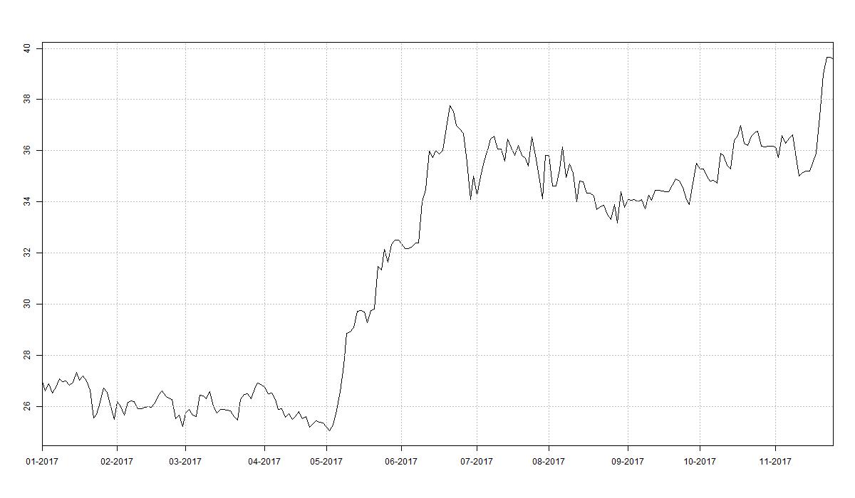
To show you some plots of various technical indicators in the following section I decided on the stock price history of Eckert Ziegler AG as a demonstration target. Eckert Ziegler AG is active in the field of isotope technology for medical, scientific and industrial use, such as cancer therapy and nuclear-medical imaging. Opening, high, low and closing prices are available on yahoo.com and are downloadable in csv format. The closing price between 2 January 2017 and 24 November 2017 is plotted below.
Indicator Examples
In the following I present some technical indicators to you which are especially common. The indicators are plotted together with the relevant price series’ of Eckert Ziegler AG. In the case where the indicator is a trading strategy the plot background is divided into green and red subsections. A green section denotes the strategy being positioning long over this period. Similarly, a red background indicates a short position.
Four Weeks Rule
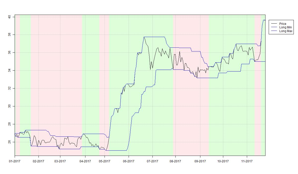
The Four Week Rule (4WR) is our first example of a trend-following trading strategy. In its basic version the strategy generates long and short signals only. The 4WR is therefore always positioned in the trading target. The rule generating signals is as follows:
- Enter into a long position and close a short position whenever the current closing price exceeds the maximum closing price of the previous four weeks.
- Enter into a short position and close a long position whenever the current closing price falls below the minimum closing price of the previous four weeks.
Crossing Moving Averages
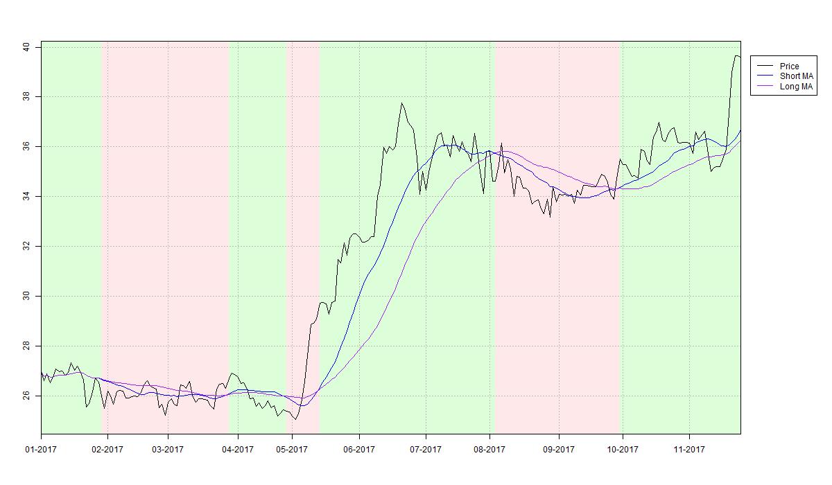
Crossing Moving Averages (XMA) are another example of a trend-following trading strategy. Long and short signals indicating a new increasing resp. decreasing trend are generated from the relative position of two moving averages on the trading target's closing price. While one could use any kind of weighted moving averages the most commonly chosen ones are two simple moving averages with window lengths of 7 and 14 days. The below plot depicts these for the case of Eckert Ziegler AG. Upward trends are identified and thus long signals are generated whenever the shorter moving average lies above the longer moving average at a particular date. Likewise, downward trends and short signals are indicated by the shorter moving average lying below the longer moving average at some date. Compare the plot to see how the 7-day moving average cuts through the 14-day moving average from below in the midst of May 2017 thereby generating a buy signal. The position is maintained until the 7-day moving average crosses the 14-day moving average from above causing the XMA strategy to enter into a short position.
Bollinger Bands
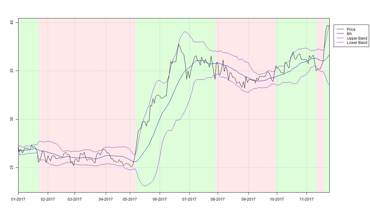
Bollinger Bands (BOL) are a trend-following trading strategy incorporating the trading target's volatility. The key idea is to require bigger price changes to generate signals during times of high volatility and similarly to allow smaller price changes to generate signals during times of low volatility. Bollinger Bands measure volatility in terms of the trading targets closing price standard deviation over a moving window of usually 20 days. The BOL indicator is constructed as follows:
- Calculate a 20 day moving average on the closing price time series.
- At each point in time add and subtract two standard volatilities over the previous 20 days to the moving average.
Average Directional Index
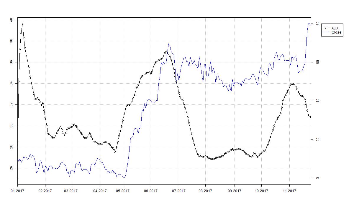
The technical indicators 4WR, XMA and BOL all aim to follow an existing price trend utilising break-out and moving average techniques. While these approaches proved decent performance in trending markets they all struggle during sideways markets. It is therefore crucial to be able to classify a market as trending or trendless. The most common instrument for this task is the Average Directional Movement Index (ADX). This technical indicator does not generate signals but rather measures the degree to which a market can be classified as trending on a scale between 0 and 100. Practitioners often consider a market trendless when the ADX is lower than 15. Equivalently, periods during which the ADX is above 15 are usually considered as trending markets. It is important to understand that the ADX does not provide any information on the actual direction of a potential trend.
As you can see, during May and July 2017, the ADX classifies the stock price of Eckert Ziegler AG as trending and trendless during the preceding and subsequent two months. Many trading systems employ the ADX indicator together with trend-following strategies like 4WR, XMA or BOL such that a long or short position in that market is taken dependent on the latter indicators, if ADX identifies a trend. During the remaining time these trading systems take a neutral position, i.e. stay off that market.
Average True Range
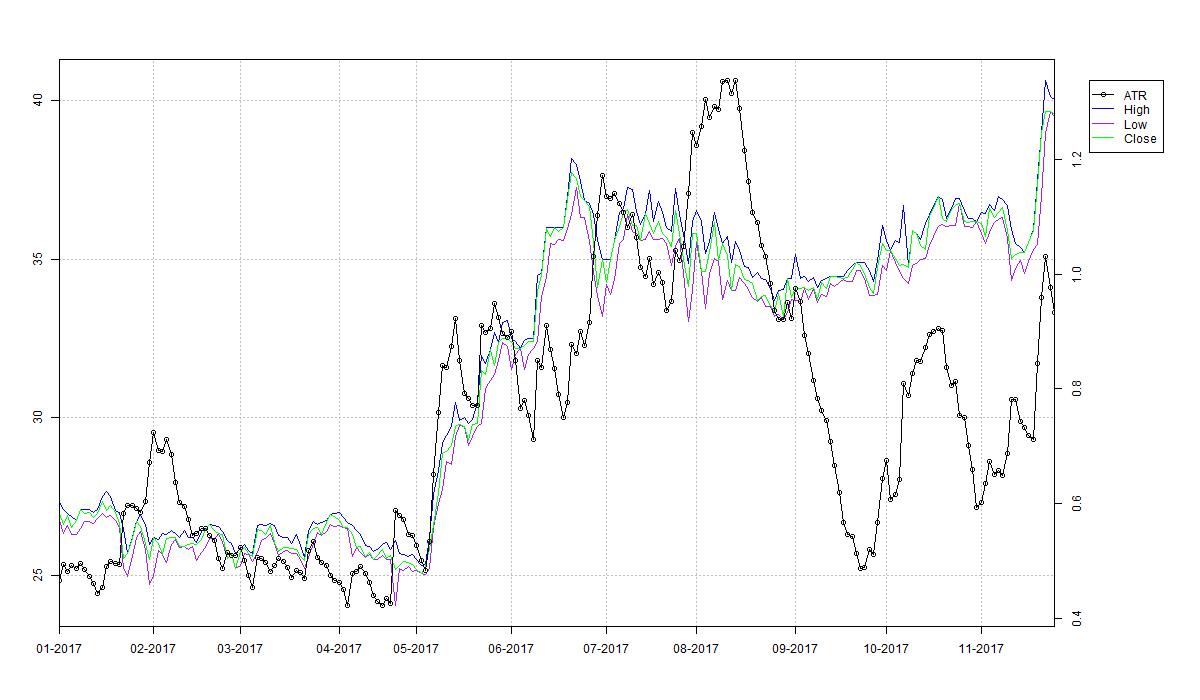
With the Bollinger Bands we already encountered the concept of adapting a trading strategy to the level of local volatility in a trading target’s price series. Another technical indicator measuring this volatility without generating signals at the same time is the Average True Range (ATR) indicator. First note that the difference of high and low price of a single trading day is called this day’s range. The True Range for this particular day is defined as the largest of
- the range, i.e. high minus low price,
- the absolute value of the day’s high minus the previous day’s close,
- the absolute value of the day’s low minus the previous day’s close.
Note that the ATR is not a trend indicator: High ATR levels do not necessarily suggest that the market is developing a trend in either direction. A large ATR just shows that the intra-day price range is large, which can be observed in both trending markets as well as volatile sideways markets. In the case of Eckert Ziegler AG the ATR is large in both the upward trend during May and June 2017 as well as in the strongly volatile sideways market during end of July and early August 2017.
Rate of Change
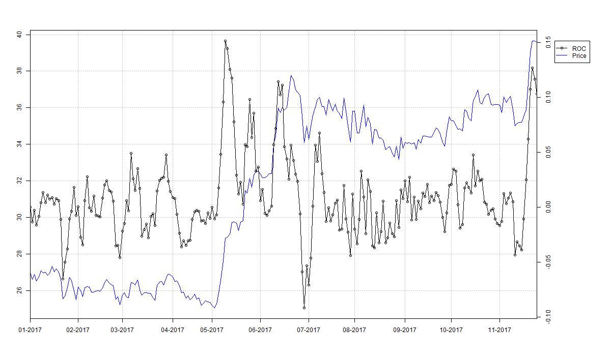
There is not too much to say about the Rate of Change (ROC) indicator. It is simply the percentage rate of change of the trading targets price series over a certain period. Especially, the ROC indicator with lag equal to one day yields the trading target’s daily return series. The ROC is therefore purely descriptive and might function as a filter for other technical indicators. For example, major price changes, such as those induced by unexpected positive earnings announcements often introduce a subsequent upward trend.
Stochastic
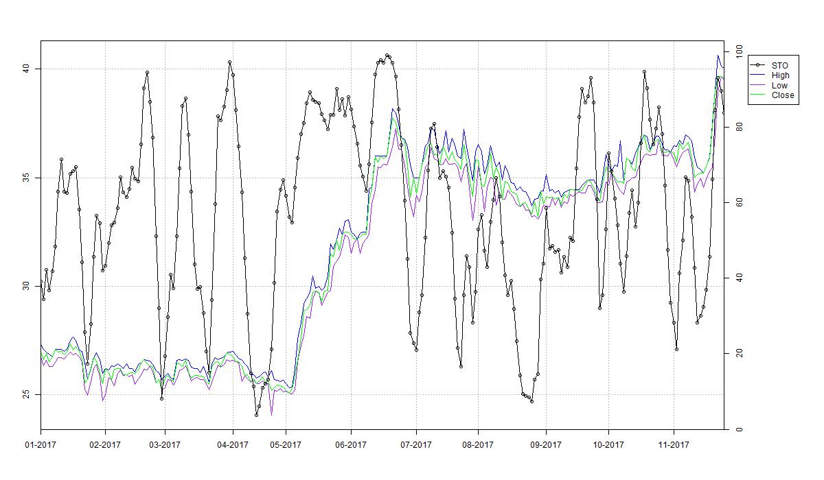
Finally, the Stochastic (STO) is an example of an oscillator. It is based upon the observation that during an upward trend closing prices tend to be close to recent highs and likewise close to the low during downward trends. Therefore, in a first step for each day the relative position of that day’s close to the previous k-day range is calculated, where k is usually set to 14 days. The result is a number between 0 and 1. Thus multiplication with 100 yields the typical oscillator scale. Plotting the resulting curve over time gives the so called %K curve. When interpreting this outcome %K values above 80 are frequently considered as an indication for an upward trend while %K values below 20 indicate a potential downward trend. To stabilise the oscillator a d-day simple moving average of the %K curve yielding the %D curve is calculated. The %D curve gives the STO oscillator, where d is often chosen to be three. Some practitioners call this version the fast Stochastic and consider a slow version defined as another d-day simple moving average of the %D curve.
Note that for mathematicians the naming “Stochastic” is not very satisfying as to them it is a synonym for the field of probability theory.
Implementation
I implemented the calculation and plotting of all indicators in R. The below code snippet serves as the main script calling all individual implementations. You may want to play with the parameters such as the moving average windows, which are set under the comment # hyper parameters. Note that the plots are directly written to jpeg files and do not occur on your R IDE.
#
# calculate and plot multiple technical indicators for sample data set
#

setwd("C:/Local/Programming/R/Trading")
rm(list=ls())

source("Indicators/TechnicalIndicators.R")

#################################################################################
# parameters
da_start        = as.Date("2017-01-01")
da_cur_date     = Sys.Date()
s_ticker        = "EckertZiegler"
s_output_dir    = "Output"

#################################################################################
# load data
df_data = read.csv(file=paste("Data/", s_ticker, ".csv", sep=""), header=TRUE, sep=",")
df_data = df_data[as.Date(df_data$Date) >= da_start, ]

head(df_data)

#################################################################################
# prepare input data
v_date  = df_data$Date
v_open  = df_data$Open
v_high  = df_data$High
v_low   = df_data$Low
v_close = df_data$Close

#################################################################################
# plot close
plotStock(v_date, v_close, paste(s_output_dir, "/", s_ticker, da_cur_date, ".jpg", sep=""))

#################################################################################
# hyper parameters
b_neutral           = FALSE
i_xma_window_short  = 20
i_xma_window_long   = 40
i_week_window_short = 10
i_week_window_long  = 20
i_bol_window        = 20
i_bol_leverage      = 2
i_atr_window        = 10
i_roc_lag           = 5
i_sto_window_k      = 10
i_sto_window_d      = 3
i_adx_window        = 20

#################################################################################
# evaluate indicators

# XMA
df_xma = XMA(v_close, i_xma_window_short, i_xma_window_long)
plotXMA(v_date, df_xma, paste(s_output_dir, "/XMA_", da_cur_date, ".jpg", sep=""))

# 4WR
df_4wr = FWR(v_close, i_week_window_short, i_week_window_long, b_neutral)
plotFWR(v_date, df_4wr, paste(s_output_dir, "/4WR_", da_cur_date, ".jpg", sep=""))

# BOL
df_bol = BOL(v_close, i_bol_window, i_bol_leverage)
plotBOL(v_date, df_bol, paste(s_output_dir, "/BOL_", da_cur_date, ".jpg", sep=""))

# ATR
df_atr = ATR(v_high, v_low, v_close, i_atr_window)
plotATR(v_date, df_atr, paste(s_output_dir, "/ATR_", da_cur_date, ".jpg", sep=""))

# STO
df_sto = STO(v_high, v_low, v_close, i_sto_window_k, i_sto_window_d)
plotSTO(v_date, df_sto, paste(s_output_dir, "/STO_", da_cur_date, ".jpg", sep=""))

# ROC
df_roc = ROC(v_close, i_roc_lag)
plotROC(v_date, df_roc, paste(s_output_dir, "/ROC_", da_cur_date, ".jpg", sep=""))

# ADX
df_adx = ADX(v_high, v_low, v_close, i_adx_window)
plotADX(v_date, df_adx, paste(s_output_dir, "/ADX_", da_cur_date, ".jpg", sep=""))
The file Indicators/TechnicalIndicators.R functions as a joint include file for all implemented technical indicators, see below for the actual content.
#
# joint import of various technical indicators
#

source("Indicators/ADX.R")
source("Indicators/ATR.R")
source("Indicators/BOL.R")
source("Indicators/ROC.R")
source("Indicators/STO.R")
source("Indicators/XMA.R")
source("Indicators/4WR.R")
For the actual implementation of the presented technical indicators refer to the series Implementing Technical Indicators. As these share several tools for plotting purposes or recurring calculations of running extrema or moving averages further source code provided in Implementing Technical Indicators: Tools has to be included. See below for a list of all relevant articles: