Kernel Density Estimation with R and Python

Introduction

In this post we will touch a variety of topics. The focus is on how to access a fast kernel density estimation implementation from within R frameworks. I therefore briefly recap the statistical concept of kernel density estimation. Then, we will come to its R implementations and see why in some instances it could be desirable to rather use an external Python implementation of kernel density estimation. We will encounter one possible way to call Python functionality from R code. Finally, I provide some example code to see kernel density estimation in such a framework in action.

Kernel Density Estimation

Imagine we are given a data sample and are interest in the underlying density. A well-known approach to describing the sample distribution is the histogram. While it is a straightforward concept, the histogram lacks continuity and smoothness. Alternatively, fitting a parametric density family will come with all the density family’s properties. But identifying a parametric density that matches the actual data well is often cumbersome if not even impossible.

Kernel density estimation (KDE) is yet another statistical non-parametric tool closely related to histograms but featuring simple density-like building blocks, the kernels. To formally introduce KDE, let \({x_1, ..., x_n}\) be the data sample, let \({h > 0}\) be the bandwidth parameter and let the kernel \({K \geq 0}\) be a function integrating to \(1\). Then \(\widehat{f}_{KDE}\) defined as follows is an estimate for the density at each \({x \in \mathbb{R}}\): \[ \widehat{f}_{KDE}(x) = \frac{1}{n} \sum_{i=1}^{n} K \left ( \frac{x - x_i}{h} \right ) \] By construction, the density estimate \(\widehat{f}_{KDE}\) integrates to one. A variety of useful kernels exists, a common example is the Gaussian kernel \(K_{\phi}\) with \[ K_{\phi}(x) = \frac{1}{\sqrt{2\pi}} e^{-\frac{1}{2}x^2} . \] Let’s briefly understand what the KDE is actually doing: The kernels approximate the data sample’s local distributional behaviour. If kernels are chosen with an unbounded support, like the Gaussian kernel, at each \({x \in \mathbb{R}}\) the density estimate \(\widehat{f}_{KDE}\) depends on all \(n\) kernels. The bandwidth parameter \(h\) controls the degree of smoothness of \(\widehat{f}_{KDE}\). Setting \({h > 0}\) to larger values results in a smoother density estimation and vice versa.

Implementations Available in R and Python

When it comes to implementations of kernel density estimation available in the R universe, quite a few packages exist out there. But how to decide among these? Besides differences in each specific KDE algorithm I consider the following two criteria especially relevant to anyone applying KDE:

1. Dimensionality of target data set: While the majority of KDE implementations are restricted to 1-dimensional data sets only, many real world applications feature higher dimensionality.
2. Performance of the implementation: One key driver of an R package’s performance is the choice of programming language in which the actual calculation logic is coded. Some R packages stick to R code only, others make use of C++ or other high-performance languages.

The authors test and benchmark the performance of 15 R packages. Out of these packages nine are designed for 1-dimensional KDE only, four are capable of 2-dimensional KDE and one package each is able to handle up to 3- respectively 6-dimensional data. According to Table 1 in their paper, ks is the R package of choice for KDE on data sets of dimensions greater than three. When working on such data sets I found ks to be too time consuming. Depending on the device a data set of \(10,000\) samples of three variables will easily take several second to be processed by ks. One possible way out is to borrow a KDE implementation from another programming language such as Python’s scipy library. The KDE functionality is implemented in stats.gaussian_kde(). By writing borrow I refer to a setup where one’s framework is written in R and at some point in the overall program logic a KDE is required.

Accessing Python functionality from R is easy. Here is one way to make scipy’s KDE version available from R: Prepare a Python script that loads a matrix from file, calls scipy’s stats.gaussian_kde() upon it and writes the result back to another csv file. Then to call this Python script from R, first store the data sample to a csv file, e.g. use R’s write.table(). Afterwards, invoke the Python script via R’s system2() function. The KDE result may than be read into R by using read.csv().

For an example of the approach described above, please see the next section.

Note, that this method of invoking Python functionality from R is transferable to other Python libraries.

Application to Simulated Data

Let us conclude with a code example on how to call Python’s KDE implementation from R. For this purpose, refer to the R and Python scripts below. If you have not already installed Python, I recommend downloading the Anaconda distribution. Do not forget to update your path variable accordingly! As the code hopefully is more or less self-explanatory, I just make a few points:

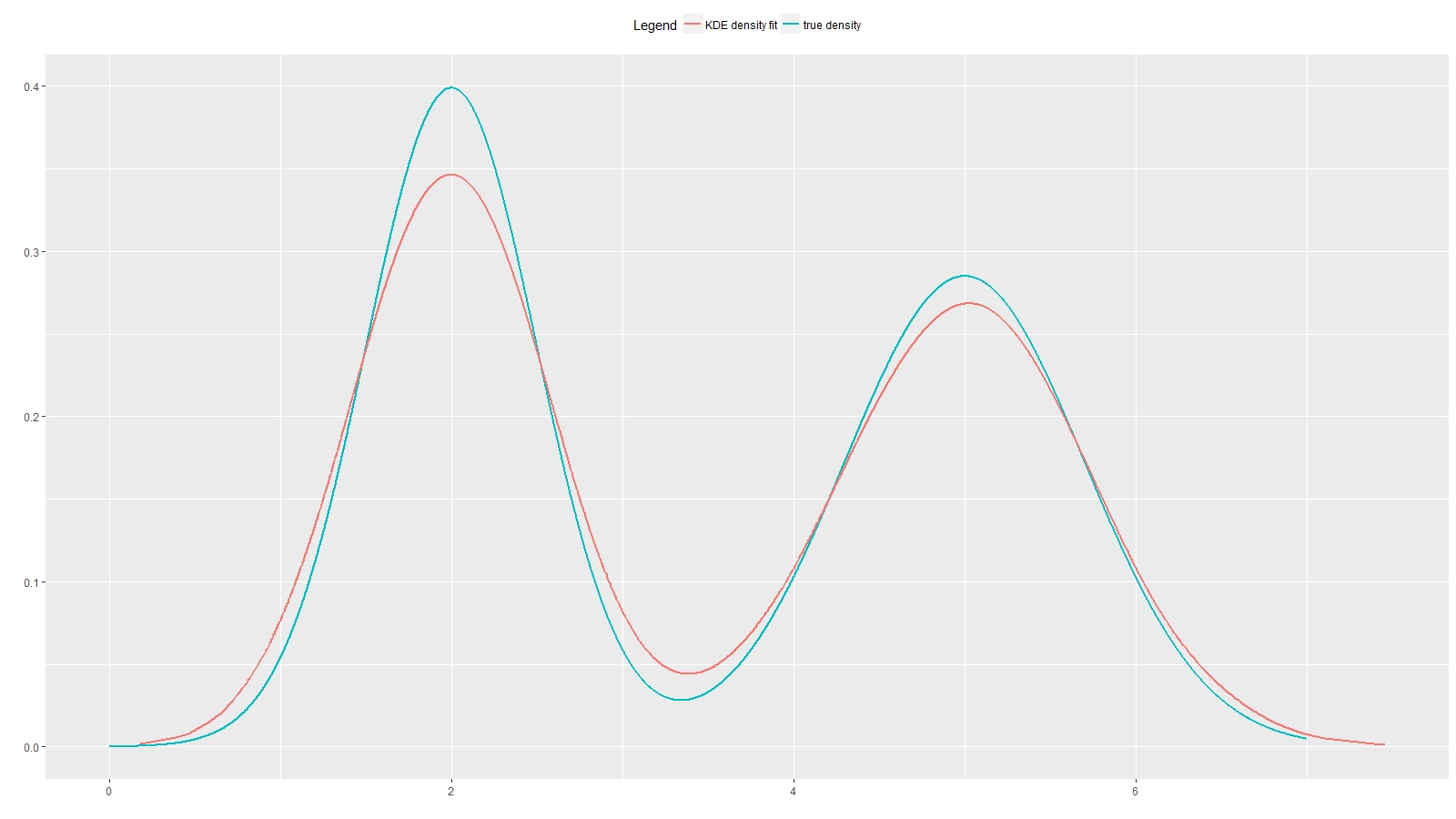
The distribution from which we sample to generate input to the kernel density estimation is chosen to be a bimodal normal mixture distribution with means \(2\) and \(5\) and standard deviations \(0.5\) and \(0.7\). Both normal distributions are equally weighted, i.e. \({\lambda_1 = \lambda_2 = 0.5}\). As a quick reminder, sampling from the mixture distribution \({p = \lambda_1 \phi(\bullet; \mu_1, \sigma_1^2) + \lambda_2 \phi(\bullet; \mu_2, \sigma_2^2)}\) can be achieved by iterating over the following two steps:

1. Randomly select one of the two mixture component 1 or 2 by drawing from a uniform distribution and selecting component 1 if the uniform sample is smaller than \(\lambda_1\). Likewise, if the uniform sample is greater than \(\lambda_1\), select component 2.
2. Draw a random sample from the selected component \({i \in \{1, 2\}}\), i.e. sample from \({\mathcal{N}(\mu_i, \sigma_i^2)}\).

library(ggplot2)

rm(list=ls())

#setwd("your/working/directory")
python_script_path <- paste0(getwd(), "/gaussian_kde.py")
python_input_file  <- paste0(getwd(), "/python_kde_input.csv")
python_output_file <- paste0(getwd(), "/python_kde_output.csv")

# define bimodel mixture distribution
lambda1 <- 0.5
lambda2 <- 0.5
mu      <- c(2, 5)
sd      <- c(0.5, 0.7)
pdf1    <- function(x) dnorm(x, mu[1], sd[1])
pdf2    <- function(x) dnorm(x, mu[2], sd[2])
pdf     <- function(x) lambda1*pdf1(x) + lambda2*pdf2(x)

# plot mixture distribution
x <- seq(0, 7, 0.001)
p <- pdf(x)

ggplot(data.frame(x, p), aes(x, p)) +
  geom_line(size=1.2) +
  xlab("") +
  ylab("")

# sample from mixture distribution
n      <- length(x)
choice <- sample(x       = c(1, 2),
                 prob    = c(lambda1, lambda2),
                 size    = n,
                 replace = TRUE)

x_sample <- rnorm(n=n, mean=mu[choice], sd=sd[choice])

# plot histogram of sampled data
ggplot(data.frame(x=x_sample), aes(x)) +
  geom_histogram(bins=30)

# Gaussian kernel density estimation via scipy
write.table(x         = x_sample,
            file      = python_input_file,
            col.names = FALSE,
            row.names = FALSE)

py_args   <- c(python_script_path,
               python_input_file,
               python_output_file)
py_result <- as.numeric(system2("python", args=py_args, stdout=TRUE))

dens_estimate <- read.csv(py_args[3], header=FALSE)$V1

# plot KDE result
index <- order(x_sample)

ggplot(data.frame(x         = x,
                  true_dens = p, 
                  x_sample  = x_sample[index],
                  kde_dens  = dens_estimate[index]),
       aes(x, true_dens)) +
  geom_line(aes(x, true_dens, colour="true density"), size=2) +
  geom_line(aes(x_sample, kde_dens, colour="KDE density fit"), size=2) +
  xlab("") +
  ylab("") +
  theme(legend.position="none")

				

# -*- coding: utf-8 -*-

#!python

import numpy as np
import pandas as pd
from scipy import stats
import sys

data   = pd.read_csv(sys.argv[1]).values.transpose()
kernel = stats.gaussian_kde(data)
index  = np.argmax(kernel.pdf(data))

print('\n'.join(data[:, index].astype(str).tolist()))