A Random Forest based Trading Strategy

Introduction

When it comes to forecasting the direction of future stock price movements usually either fundamental or technical analysis is applied. As corporations publish financial statements only a few times a year fundamental analysis is less applicable to short-term stock price forecasting. Technical analysis on the other hand operates on much more granular data, i.e. historical stock price data. In this article I will develop a trading strategy based on the theory of technical indicators and modern machine learning techniques. The focus is on bringing together a variety of concepts rather than coming up with the definite trading strategy – sorry.

If you are knew to technical indicators I recommend to first check on my corresponding article Technical Indicators: An Introduction. There I present a list of indicators and oscillators, each allowing to either classify market conditions or estimating the underlying trend’s direction. Although in the article mentioned above the four week rule, crossing moving averages and Bollinger bands do all reasonable good at identifying the sharp price increase (May 2017) in the article’s example data, none of them is able to consistently detect all trend changes. So why not try to combine several indicators to create a potentially superior one? An easy to handle machine learning algorithm for this task is random forest learning. I will briefly recap on random forests below before introducing the actual trading strategy.

Note that (nonlinear) time series analysis would be the canonical approach to predicting a stock’s future price development.

Random Forests & Implementation in R

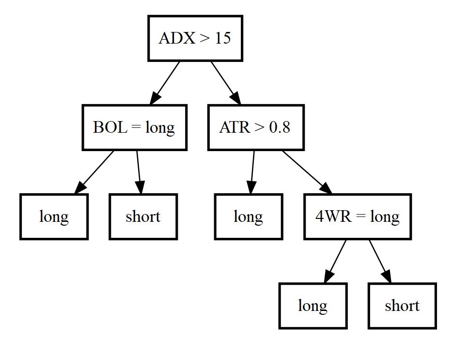
Let’s briefly recap on random forests as one of today’s most popular regression and especially classification machine learning algorithms: As the name already gives away, a random forest consists of multiple tree structures. Each such tree itself is a regression or classification algorithm. The structure of a single tree is learned by iteratively selecting features upon whose dimension the feature space is splitted with respect to a certain optimality criteria. As a result of iteratively conditioning on other features, the resulting tree structure introduces nonlinearity to regression and classification. Popular tree learning frameworks are CART and C4.5. We will see an example for a classification tree in the following section.

Random forests now combine multiple trees in order to minimise prediction error. They are therefore an example of an ensemble learning algorithm. In order to get a single prediction from the ensemble of trees in a regression setup the individual tree’s predictions are averaged whereas for classification tasks a majority vote among all trees is conducted. But how can we grow a set of differing trees on a single data sample? This is where bagging (“bootstrap aggregation”) comes in: For each tree to be learned a learning sample is generated by sampling data uniformly with replacement from the original data set. As a result, individual trees will come up with different features selected and different split locations. Much more can be said about random forests, but here this is about how much we need to know in order to come up with our trading strategy.

One of the fastest implementations of the random forest framework available for R which I know off is the ranger package. It gains a performance advantage over other packages from its efficient C++ implementation. For further details on the implementation and performance comparison with other packages I recommend to have a look at the authors’ original paper.

The Trading Strategy

The trading strategy’s underlying model is built upon the following four blocks:

1. Data: The data available for this task are the time series of daily opening and closing prices as well as each day’s high and low, i.e. the maximum and minimum quotes respectively.
2. Feature extraction: From the price data we derive features for our model by calculating the following technical indicators:
   • 4WR: Four Weeks Rule
   • XMA: Crossing Moving Averages
   • BOL: Bollinger Bands
   • ADX: Average Directional Index
   • ATR: Average True Range
   • ROC: Rate of Change
   • STO: Stochastic
   Further details on these technical indicators can be found in my article Technical Indicators: An Introduction. It also refers to an R implementation.
3. The target variable: For each day calculate the return of close price over the following five trading days. If the result is greater than zero, store the signal 1, otherwise, store 0. By constructing such a signal target variable we try to keep the number and therefore cost of trading within bounds.
4. The model: Given technical indicator values derived from the historical price quotes we aim at predicting whether prices will increase or decrease over the next week. If prices are predicted to increase, the strategy enters a long position. Likewise, if prices are predicted to decrease, the strategy enters a short position. As this is a classification task (with classes 0 and 1) we can learn a classifier with the random forest framework described in the previous section.

Data Preparation

Business before pleasure: We apply the implementations of all technical indicators as covered in my series Implementing Technical Indicators to prepare data. The two relevant source files are IndicatorPlottingFunctions.R and TechnicalIndicators.R. Data can be downloaded from yahoo.com in csv format and shall be placed in a subfolder called data of your working directory. I chose stock price quotes for Eckert Ziegler AG during the period of 2 January 2017 to 24 November 2017. The following code imports the csv file, extracts price time series and constructs all technical indicator values. Parameters to the technical indicators are hyperparameters to our random forest based trading strategy, i.e. they are not subject to the random forest fitting. Note that these could be tuned themselves, which I will not cover in this article.

rm(list=ls())

# import
source("Indicators/TechnicalIndicators.R")

# helper function
custom_trim = function(v, lag) {
  return(v[-c(1, ((length(v)-lag+1):length(v)))])
}


#################################################################################
# parameters
da_start         = as.Date("2017-01-01")
da_cur_date      = Sys.Date()
s_ticker         = "EckertZiegler"
s_output_dir     = "Output"
i_prediction_lag = 5


#################################################################################
# hyper parameters
# available strategies: 4WR, ADX, ATR, BOL, ROC, STO, XMA
b_neutral           = FALSE
i_xma_window_short  = 20
i_xma_window_long   = 40
i_week_window_short = 10
i_week_window_long  = 20
i_bol_window        = 20
i_bol_leverage      = 2
i_atr_window        = 10
i_roc_lag           = 5
i_sto_window_k      = 10
i_sto_window_d      = 3
i_adx_window        = 20


#################################################################################
# load data

# load training data
df_data = read.csv(file=paste("data/", s_ticker, ".csv", sep=""), header=TRUE, sep=",")
df_data = df_data[as.Date(df_data$Date) >= da_start, ]

head(df_data)


#################################################################################
# prepare input data
v_date  = df_data$Date
v_open  = df_data$Open
v_high  = df_data$High
v_low   = df_data$Low
v_close = df_data$Close


#################################################################################
# prepare dependent variable:
# - 1: price increases during subsequent n days
# - 0: price decreases during subsequent n days
v_direction = n_lag_direction(v_close, i_prediction_lag)


#################################################################################
# prepare training sample
df_training = data.frame(
                adx = ADX(v_high, v_low, v_close, i_adx_window)$ADX,
                atr = ATR(v_high, v_low, v_close, i_atr_window)$ATR,
                bol = BOL(v_close, i_bol_window, i_bol_leverage)$Signal,
                fwr = FWR(v_close, i_week_window_short, i_week_window_long, b_neutral)$Signal,
                roc = ROC(v_close, i_roc_lag)$ROC,
                sto = STO(v_high, v_low, v_close, i_sto_window_k, i_sto_window_d)$STO,
                xma = XMA(v_close, i_xma_window_short, i_xma_window_long)$Signal,
                dir = factor(v_direction)
              )

df_training   = df_training[-c(1, ((length(v_close)-i_prediction_lag+1):length(v_close))), ]
v_close_train = custom_trim(v_close, i_prediction_lag)
v_date_train  = custom_trim(v_date,  i_prediction_lag)

head(df_training)

				

Implementing the Trading Strategy

Fitting the Random Forest

I decided to use the ranger package for learning the random forest. All we have to do is pass df_training to the ranger function. As we want to explain the direction dir of future price movements by the values of all our technical indicators we specify dir ~ . as our model, where the period indicates all variables in data except for the target variable. Note that we made dir a factor during data preparation to let ranger know that it has to handle a classification task. The other two arguments provided are "permutation" as importance measure and a seed of 99. I will address the importance measure parameter below. Further, it is always good to set a seed when there is randomness included in the algorithm to allow for reproducibility: Remember that the samples selected as in-bag for each tree are drawn uniformly with replacement from the full data sample.

library(ranger)

#################################################################################
# fit HL_RandomForest on training sample
hl_strategy = ranger(dir ~ .,
                     data       = df_training,
                     importance = "permutation",
                     seed       = 99)

				

Assessing the Model

It is now time to examine the goodness of fit of our random forest model. Assessing a prediction model’s fit should always include in-sample as well as out-of-sample goodness measures. The below code calculates the in-bag and out-of-bag errors. Some recurring helper functionality is implemented in a separate file backtesting.R of which you find the code below as well. Finally, additional data for the period from 2 January 2018 to 3 August 2018 is imported and the previously learned model hl_strategy is evaluated on the new data.

The in-bag misclassification rate turns out to be 0%. This is not surprising as random forests usually manage to fit the as in-bag selected samples (nearly) perfectly. Of much greater interest is hl_strategy$prediction.error, the out-of-bag misclassification rate which is a measure for the model’s generalisation error and takes a value of 29.6%.

# import
source("strategy/backtesting.R")

s_ticker_test = "EckertZiegler2"


#################################################################################
# evaluate HL_RandomForest fit:
v_predictions = predictions(predict(hl_strategy, data=df_training))
v_signals_train = class_to_signal(as.numeric(as.vector(v_predictions)))

v_strategy_train  = eval_performance(v_close_train, v_signals_train)
i_position_swings = count_position_swings(v_signals_train)

# 1. in-bag training error
print(table(class_to_signal(as.numeric(as.vector(df_training$dir))), v_signals_train))

# 2. out-of-bag error
print(hl_strategy$prediction.error)


#################################################################################
# load test data
df_data_2 = read.csv(file=paste("data/", s_ticker_test, ".csv", sep=""), header=TRUE, sep=",")
df_data_2 = df_data_2[df_data_2$Close != "null", ]

head(df_data_2)


#################################################################################
# evaluate HL_RandomForest performance on test sample
v_date_test  = df_data_2$Date
v_close_test = as.numeric(as.vector(df_data_2$Close))
v_high_test  = as.numeric(as.vector(df_data_2$High))
v_low_test   = as.numeric(as.vector(df_data_2$Low))

v_direction_test = custom_trim(n_lag_direction(v_close_test, i_prediction_lag), i_prediction_lag)

df_test = data.frame(
  adx = ADX(v_high_test, v_low_test, v_close_test, i_adx_window)$ADX,
  atr = ATR(v_high_test, v_low_test, v_close_test, i_atr_window)$ATR,
  bol = BOL(v_close_test, i_bol_window, i_bol_leverage)$Signal,
  fwr = FWR(v_close_test, i_week_window_short, i_week_window_long, b_neutral)$Signal,
  roc = ROC(v_close_test, i_roc_lag)$ROC,
  sto = STO(v_high_test, v_low_test, v_close_test, i_sto_window_k, i_sto_window_d)$STO,
  xma = XMA(v_close_test, i_xma_window_short, i_xma_window_long)$Signal
)

df_test      = df_test[-c(1, ((length(v_close_test)-i_prediction_lag+1):length(v_close_test))), ]
v_close_test = custom_trim(v_close_test, i_prediction_lag)
v_date_test  = custom_trim(v_date_test,  i_prediction_lag)

v_predictions_test = predictions(predict(hl_strategy, data=df_test))
v_signals_test     = class_to_signal(as.numeric(as.vector(v_predictions_test)))
v_strategy_test    = eval_performance(v_close_test, v_signals_test)

print(table(class_to_signal(as.numeric(as.vector(v_direction_test))), v_signals_test))

				

#
# backtesting utilities for trading strategies
#

eval_performance = function(price, signal) {
  return(cumsum(c(price[1], diff(price, 1) * signal[1:(length(signal)-1)])))
}

count_position_swings = function(signal) {
  return(sum(diff(signal, 1) != 0))
}

class_to_signal = function(signal) {
  return(2*signal - 1)
}

n_lag_direction = function(price, lag) {
  n_diff = c(diff(price, lag), rep(1, lag))
  y = rep(1, length(price))
  y[n_diff >= 0] = 1
  y[n_diff <  0] = 0

  return(y)
}

				

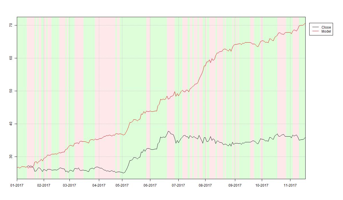
So how does the random forest misclassification analysis relate to performance of the learned trading strategy on Eckert Ziegler AG stock price data? We just take the model predicted trading signals for in-sample (2017-01-02 to 2017-11-24) as well as out-of-sample (2018-01-02 to 2018-08-03) prices and plot the related performance versus a simple buy-and-hold strategy over the respective period. The first plot below shows the in-sample performance with a whopping 166% return over the year 2017. If you are impressed by this performance it is likely that you are among the target customers of Financial Times’ Hindsight Capital LLC.

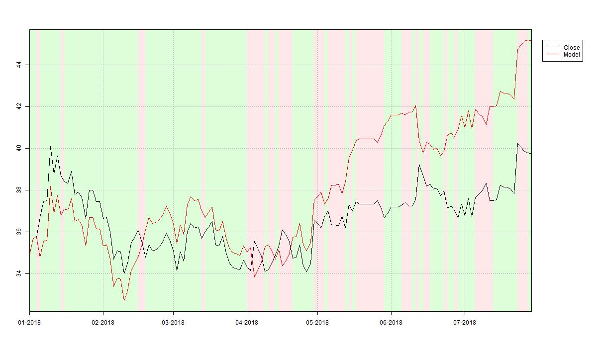
Further – and now serious again – the second plot below shows the random forest based trading strategy’s out-of-sample performance over the first eight months of year 2018. The strategy materialises an outperformance of 15% over a buy-and-hold strategy over the same period. This is largely due to good performance on the test period’s second half.

The code used to create the two above plots is printed below. For the source code of IndicatorPlottingFunctions.R refer to my article Implementing Technical Indicators: Tools.

#import
source("Indicators/IndicatorPlottingFunctions.R")


#################################################################################
# visualise performance

# plot training sample performance
plotIndicator(v_date_train,
              v_signals_train,
              data.frame(close = v_close_train,
                         model = v_strategy_train),
              c("black", "red"),
              c("Close", "Model"),
              paste0(s_output_dir, "/HL_RandomForest_", da_cur_date, "_train", ".jpg"))

# plot test sample performance
plotIndicator(v_date_test,
              v_signals_test,
              data.frame(close = v_close_test,
                         model = v_strategy_test),
              c("black", "red"),
              c("Close", "Model"),
              paste0(s_output_dir, "/HL_RandomForest_", da_cur_date, "_test", ".jpg"))

				

Feature Importance

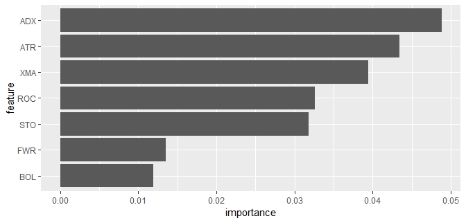
For statistical models such as classical OLS linear regression it is common to examine the impact of individual features on prediction. Unfortunately, as machine learning models such as random forests usually introduce a highly nonlinear relationship between features and target variable, in their case the measurement of feature importance is non-trivial. A common method for gaining insights into the relative importance of features in machine learning frameworks is feature permutation. The underlying concept is simple: Take a single feature and shuffle its sample values to break any relationships with other data while keeping all other feature’s values in order. Then rerun the model and compute the increase in prediction error. The greater that increase is, the more relevant the feature is considered.

The below code creates a bar chart depicting each technical indicator’s importance by means of feature permutation. We find the ADX indicator to be reported most relevant and the BOL indicator least relevant. We now have to be careful with interpretation of this relation: The trading strategy’s predictive power stems from allowing all features to operate together in tree structures. So no single indicator is sufficiently good at outperforming the trading target. As depicted in the tree example above, individual indicators are more meaningful in certain market regimes, e.g. trend-following strategies such as XMA perform better in trending markets for obvious reasons. Thus I read the feature importance plot for our random forest based trading strategy as supporting this idea by selecting the trend strength measurement indicator ADX as the most relevant one. To me this is the most enlightening and satisfying outcome of this little project.

library("ggplot2")

feature_importance = importance(hl_strategy)

ggplot(data.frame(feature    = toupper(names(feature_importance)),
                  importance = as.vector(feature_importance)),
       aes(x=reorder(feature, importance), y=importance)) +
  geom_bar(stat="identity") +
  coord_flip() +
  xlab("feature")

				

Ideas for Future Improvement

As mentioned in the introduction, the purpose of this project was to show how random forests could be applied to stock market prediction with a focus on how individual components such as model conception, data preparation, model fitting and model evaluation are designed. Please do not consider this as an attempt to construct a perfect trading system.

I can think of quite a few interesting future improvements and research ideas to the random forest trading strategy:

1. Fit the model on price data of multiple stocks simultaneously to allow for better generalisation when applied to previously unknown stocks (transfer learning).
2. Fine-tune hyperparameters as I set them to more or less arbitrary values. Also, including the same indicator multiple times with different parameters could be valuable too, e.g. have two XMA indicators with differing moving window lengths.
3. Track performance of trading strategy over longer out-of-sample period to test for systematic outperformance.
4. Implement and add new technical indicators to account for additional market regimes.